Image by Editor

Real-world data often show particular patterns or behaviors that can be modeled by a probability distribution, a specific mathematical form that captures the uncertainty, variability, and other properties underlying the data. However, more often than not, practitioners may be unsure which distribution best fits their situation. This article provides a practical guide to help you navigate the choice of probability distributions for different types of data and analysis contexts.

Outline of the Decision Tree

The choice of the right probability distribution for modeling and performing analyses over your data largely depends on the very nature of your data and the type of information collected in it. Roughly speaking, in terms of probability distributions, we can distinguish among three types of data, as shown in the following decision tree diagram.

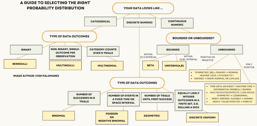
Let’s examine each of these three major options or data types in more detail, diving deeper into further questions that lead us to the right probability distribution.

Categorical Data

Categorical data can roughly belong to three different subtypes: binary data, i.e., data with two possible outcomes like yes/no or success/failure; non-binary single outcomes like color or blood type; and counts per category over a number n of trials, which is common in survey responses tallied across multiple options or when rolling a die repeatedly.

The first subtype is typically modeled using a Bernoulli distribution, whereas the second is best modeled using the Multinoulli distribution: a generalization of the Bernoulli distribution that assigns a probability to every mutually exclusive category, e.g., bird species. Finally, for modeling category counts over n trials, it makes sense to use a probability distribution like the Multinomial, which provides the probability of observing a specific combination of category counts when the n trials are independent and abide by the same categorical probabilities.

Discrete Numeric Data

Having numeric data doesn’t necessarily mean that the data are continuous. In fact, real-world examples like the number of website visits per day and the number of faulty products in a batch are discrete in nature. In this case, we distinguish among four types of data outcomes:

• Number of successes (or positive binary outcomes) in n trials: for instance, when counting how many times a coin lands heads after 10 flips. This type of outcome is best modeled by a Binomial distribution.
• Number of events within a fixed time or space interval: for instance, when counting the number of customers arriving at a store per hour. This type of outcome is best modeled by a Poisson distribution.
• Number of failed trials until the first success: for instance, when recording how many times a machine fails before producing a correct item for quality control purposes. This type of outcome is best modeled by a Geometric distribution.
• Equally probable integer outcomes in a finite set: for instance, when rolling a fair die where each face has the same likelihood. This type of outcome is best modeled by a Discrete Uniform distribution. Do not mistake this scenario for the previously mentioned one of category counts (number of times each die result was obtained), which should use a Multinomial instead of Discrete Uniform.

Continuous Numeric Data

Last, when data are numeric and continuous in nature, i.e., real numbers, we also have several sub-variants or specific situations.

If data values are bounded, they may be values like probabilities or likelihoods, bounded to the [0,1] interval, in which case the Beta distribution is often adequate, as it flexibly models distribution shapes from uniform to highly skewed. Meanwhile, if the values are bounded to any other interval [a,b], then the right approach is the Uniform distribution, assuming all values are equally probable within that range.

For unbounded (or semi-bounded) data, the range of choices is slightly wider, and it will mainly depend on whether data values can be positive and negative, or only positive.

• For data that can be positive or negative, we have the well-known Normal (Gaussian) distribution, which is well-suited for modeling phenomena like measurement errors or natural variations in specimen observations, in which data cluster symmetrically around a mean. For heavier tails, as in financial returns or datasets with outliers, the Student’s t distribution provides a better fit. For skewed data, consider the Skew-Normal; for a sharper peak with heavier tails while remaining symmetric, the Laplace distribution is a useful alternative.
• For positive-only data, we could be measuring different phenomena — for instance, the time until an event occurs, like the precise lifespan of a component (Exponential, Weibull, or Gamma distributions are suitable choices). If instead we are accounting for multiplicative effects or variables that become symmetric after taking logarithms, the Lognormal distribution fits well; whereas for right-skewed data with a few unduly large values, the Gamma again provides flexibility. Finally, for heavy-tailed positive data like wealth distributions or city population sizes, the Pareto distribution is an appropriate choice.

Wrapping Up

This article explained how to reliably select the right probability distribution for your real-world problem and collected data: to make things easier and intuitive, a decision tree has been used as a guide to lead you toward the right choice.