
 Image by Author | Ideogram
A cornerstone concept in statistics and data analysis is that of probability distributions. Understanding probability distributions is key for analysts in modeling many real-world phenomena, making predictions including those driven by machine learning models, and drawing informed insights from data. This article is your ultimate guide to understanding them gently and illustratively.
Ready to start?
What are Probability Distributions?
A probability distribution describes how probabilities are distributed across the different values or outcomes of a (random) variable. It shows how likely the different values or outcomes are, highlighting the most and least probable outcomes.
Since a random variable can be discrete (e.g. the number of children in a family) or continuous (e.g. the price of a flight ticket), probability distributions can also be either discrete or continuous.
Three key related concepts associated with probability distributions include:
1. Probability Mass Function (PMF): associated with discrete variables, the PMF gives the probabilities for individual outcomes, for example, the probability of a family having one child, having two children, and so on. Assuming X is a random variable like the number of children in a family, and x is a specific value for X, then the PMF is denoted by F(X)=P[X=x].
2. Probability Density Function (PDF): associated with continuous variables, the PDF describes the likelihood of a value falling within a range, for instance probability of a person’s height falling between 5.5 feet and 6 feet. Following a similar notation, the PDF is denoted by F(X)=P[x<=X<=x’], with x<x’.
3. Cumulative Distribution Function (CDF): it indicates the cumulated probability up to a certain value, for example, the probability of a newborn baby weighing up to 2.5kg. It is denoted by F(x)=P[X≤x].
These three functions are visually represented through the below examples:

Don’t worry if you are unfamiliar with terms like binomial and normal in the above visualizations. We will look at those next!
Common Probability Distributions
Time to make a tour of five of the most well-known probability distributions, their characteristics, and how they visually look. Real-world data and phenomena may sometimes resemble either one of these distributions, although this is not always the case with more complex datasets or variables.
1. Binomial Distribution
The purpose of a binomial distribution is to model the number of successes or positive outcomes (understood in a scenario where there are two types of outcomes: positive vs negative) after n independent trials. A common example of phenomena that follow a binomial distribution consists of tossing a coin several times, e.g. n=10 times, and determining the probability of getting x heads, with x being equal or lower than n.
The shape of this discrete distribution is typically symmetric when both possible outcomes have equal probability p=0.5 (e.g. tossing a well-shaped coin), and are skewed otherwise.

2. Poisson Distribution
This discrete probability distribution is used for describing the number of events that occur in a fixed time lapse or space, for instance, the number of calls received at a help center per hour. In a Poisson distribution, a parameter λ denotes the average rate of occurrences in a time interval, also called the expected value of the distribution. The larger the λ, the more the distribution is shifted to the right.

3. Uniform Distribution
The simplest of all continuous probability distributions, the uniform distribution describes outcomes that will equal probabilities, e.g. the probability of drawing a ball out of a bingo drum, assuming all balls numbered 1 to 99 are equally likely to be drawn.

4. Normal Distribution
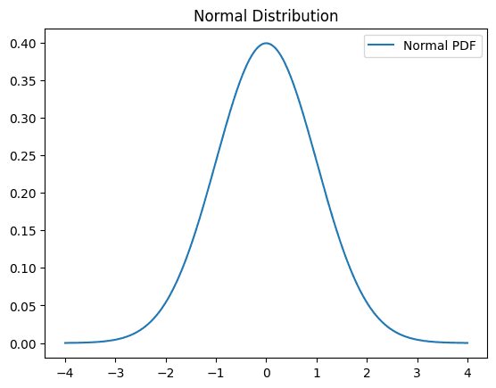
Also called Gaussian distribution, this is undoubtedly the most widely used distribution because it resembles many real-world phenomena and data. It represents data as a bell-shaped curve where most probable values are centered around the mean, denoted by μ. Another important parameter in a normal distribution is its standard deviation σ, which indicates how concentrated or spread the data are around the mean: larger σ yield wider bell-shaped curves, and vice versa. An example of data following a normal distribution is adult people’s heights, where intermediate heights are those around which most of the population falls.
5. Exponential Distribution
The exponential distribution is used to model the time between events in a process usually modeled by a Poisson distribution. Smaller values are usually more likely. An example of this is modeling the time between consecutive customer arrivals at a store, where larger time lapses between arrivals are more and more unlikely.

Wrapping Up
This article has provided an introductory guide to understanding probability distributions — a central resource, and a powerful set of tools for data analysts and practitioners to understand and model data and real-world phenomena. Different probability distributions have been defined as a result of centuries of research to model different types of random phenomena, each with their characteristics. While this article introduced five of them, many more types of probability distributions suit more specific patterns.

educative